torchcvnn.datasets
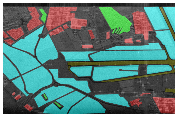
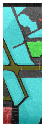
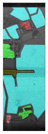
Bretigny
- class torchcvnn.datasets.Bretigny(root: str, fold: str, transform=None, balanced: bool = False, patch_size: tuple = (128, 128), patch_stride: tuple | None = None)[source]
Bretigny Dataset
- Parameters:
root – the root directory containing the npz files for Bretigny
fold – train (70%), valid (15%), or test (15%)
transform – the transform applied the cropped image
balanced – whether or not to use balanced labels
patch_size – the dimensions of the patches to consider (rows, cols)
patch_stride – the shift between two consecutive patches, default:patch_size
PolSF
- class torchcvnn.datasets.PolSFDataset(root: str, transform=None, patch_size: tuple = (128, 128), patch_stride: tuple | None = None)[source]
The Polarimetric SAR dataset with the labels provided by https://ietr-lab.univ-rennes1.fr/polsarpro-bio/san-francisco/
We expect the data to be already downloaded and available on your drive.
- Parameters:
root – the top root dir where the data are expected
transform – the transform applied the cropped image
patch_size – the dimensions of the patches to consider (rows, cols)
patch_stride – the shift between two consecutive patches, default:patch_size
Note
An example usage :
import torchcvnn
from torchcvnn.datasets import PolSFDataset

def transform_patches(patches):
    # We keep all the patches and get the spectrum
    # from it
    # If you wish, you could filter out some polarizations
    # PolSF provides the four HH, HV, VH, VV
    patches = [np.abs(patchi) for _, patchi in patches.items()]
    return np.stack(patches)

dataset = PolSFDataset(rootdir, patch_size=((512, 512)), transform=transform_patches
X, y = dataset[0]
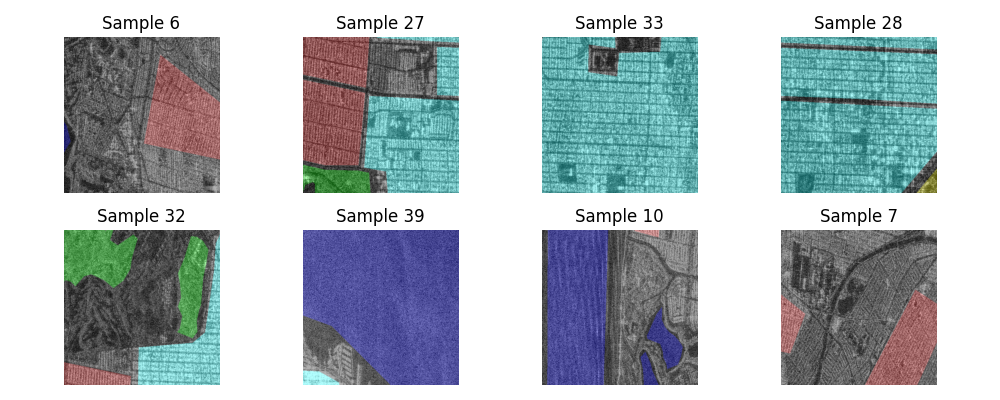
Displayed below are example patches with patch sizes \(512 \times 512\) with the labels overlayed
ALOS2
We provide a generic class for parsing ALOS2 data which is the format developed by the Japanese Aerospace Exploration Agency (JAXA).
- class torchcvnn.datasets.ALOSDataset(volpath: str | None = None, transform=None, crop_coordinates: tuple | None = None, patch_size: tuple = (128, 128), patch_stride: tuple | None = None)[source]
Bases:
DatasetThe format is described in https://www.eorc.jaxa.jp/ALOS/en/alos-2/pdf/product_format_description/PALSAR-2_xx_Format_CEOS_E_g.pdf
The dataset is constructed from the volume file. If leader and trailer files are colocated, they are loaded as well.
Important, this code has been developed for working with L1.1 HBQ-R Quad Pol datafiles. It is not expected to work out of the box for other levels and for less than 4 polarizations.
- Parameters:
volpath – the path to the VOLUME file
transform – the transform applied the cropped image. It applies on a dictionnary of patches {‘HH’: np.array, ‘HV’: np.array}
crop_coordinates – the subpart of the image to consider as ((row_i, col_i), (row_j, col_j)) defining the corner coordinates
patch_size – the dimensions of the patches to consider (rows, cols)
patch_stride – the shift between two consecutive patches, default:patch_size
This class itself involves several parsers to process the :
volume file
torchcvnn.datasets.alos2.VolFileleader file
torchcvnn.datasets.alos2.LeaderFile,image file
torchcvnn.datasets.alos2.SARImage,trailer file
torchcvnn.datasets.alos2.TrailerFile.
- class torchcvnn.datasets.alos2.VolFile(filepath: str | Path)[source]
Processing a Volume Directory file in the CEOS format. The parsed informations can be accessed through the attributes descriptor_records, file_pointer_records and text_records
- Parameters:
filepath – the path to the volume directory file
SLC
SLC is popular remote sensing format. The Nasa Jet Lab UAV SAR mission for example provides several SLC stacks.
- class torchcvnn.datasets.SLCDataset(rootdir: str | None = None, transform=None, patch_size: tuple = (128, 128), patch_stride: tuple | None = None)[source]
Bases:
DatasetThe format is described in https://uavsar.jpl.nasa.gov/science/documents/stack-format.html
This object does not download the data for you, you must have the data on your local machine. For example, you can register and access data from the NASA JetLab https://uavsar.jpl.nasa.gov
Note the datafiles can be quite large. For example, the quad polarization from Los Angeles SSurge_15305 is a bit more than 30 GB. If you take the downsampled datasets 2x8, it is 2GB.
Note the 1x1 is 1.67 m slant range x 0.6 m azimuth.
Note
As an example, using the example read_slc.py, with the SSurge_15305 stack provided by the UAVSar, the Pauli representation of the four polarizations is shown below :
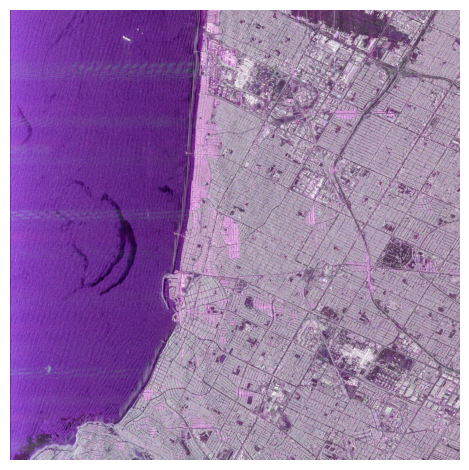
The code may look like this :
import numpy as np
import torchcvnn
from torchcvnn.datasets.slc.dataset import SLCDataset

def get_pauli(data):
    # Returns Pauli in (H, W, C)
    HH = data["HH"]
    HV = data["HV"]
    VH = data["VH"]
    VV = data["VV"]

    alpha = HH + VV
    beta = HH - VV
    gamma = HV + VH

    return np.stack([beta, gamma, alpha], axis=-1)


patch_size = (3000, 3000)
dataset = SLCDataset(
    rootdir,
    transform=get_pauli,
    patch_size=patch_size,
)
- Parameters:
rootdir – the path containing the SLC and ANN files
transform – the transform applied to the patches. It applies on a dictionnary of patches {‘HH’: np.array, ‘HV’: np.array, …}
patch_size – the dimensions of the patches to consider (rows, cols)
patch_stride – the shift between two consecutive patches, default:patch_size
This class involves several parsers for parsing :
the annotation file
torchcvnn.datasets.slc.ann_file.AnnFilethe SLC files
torchcvnn.datasets.slc.slc_file.SLCFile
- class torchcvnn.datasets.slc.ann_file.AnnFile(filename)[source]
From the documentation :
The annotation file (.ann) is a keyword/value ASCII file in which the value on the right of the equals sign corresponds to the keyword on the left of the equals sign. The number of keywords may change with time, so the line number should not be assumed to be constant for any given keyword.
In addition, the spacing between keywords and values may change. The units are given in parenthesis between the keyword and equal sign, and may change from annotation file to annotation file and within each annotation file.
Comments are indicated by semicolons (;), and may occur at the beginning of a line, or at the middle of a line (everything after the semicolon on that line is a comment). The length of each text line is variable, and ends with a carriage return. There may be lines with just a carriage return or spaces and a carriage return.
- class torchcvnn.datasets.slc.slc_file.SLCFile(filename: str, patch_size: tuple, patch_stride: tuple | None = None)[source]
Reads a SLC file
The filenames contain interesting information:
{site name}_{line ID}_{flight ID}_{data take counter}_{acquisition date}_{band}{steering}{polarization}_{stack_version}… _{baseline correction}_{segment number}_{downsample factor}.slc
e.g. SSurge_15305_14170_007_141120_L090HH_01_BC_s1_1x1.slc is
site_name : SSurge
line ID : 15305
flight ID : 14170
data take counter : 007
acquisition date : 141120, the date is in YYMMDD format (UTC time).
band : L
steering : 090
polarization : HH
stack version : 01
baseline correction : BC, means the data is corrected for residual baseline
segment number : s1
downsample factor : 1x1
There is one SLC file per segment and per polarization.
S1SLC
S1SLC is a dataset built from Sentinel-1 SLC data. The dataset is provided at the following url `https://ieee-dataport.org/open-access/s1slccvdl-complex-valued-annotated-single-look-complex-sentinel-1-sar-dataset-complex`_.
- class torchcvnn.datasets.S1SLC(root, transform=None, lazy_loading=False)[source]
Bases:
DatasetThe Polarimetric SAR dataset with the labels provided by https://ieee-dataport.org/open-access/s1slccvdl-complex-valued-annotated-single-look-complex-sentinel-1-sar-dataset-complex
We expect the data to be already downloaded and available on your drive.
- Parameters:
root – the top root dir where the data are expected. The data should be organized as follows: Sao Paulo/HH.npy, Sao Paulo/HV.npy, Sao Paulo/Labels.npy, Houston/HH.npy, Houston/HV.npy, Houston/Labels.npy, Chicago/HH.npy, Chicago/HV.npy, Chicago/Labels.npy
transform – the transform applied the cropped image
lazy_loading – if True, the data is loaded only when requested. If False, the data is loaded at the initialization of the dataset.
Note
An example usage :
import torchcvnn
from torchcvnn.datasets import S1SLC

def transform(patches):
    # If you wish, you could filter out some polarizations
    # S1SLC provides the dual HH, HV polarizations
    patches = [np.abs(patchi) for _, patchi in patches.items()]
    return np.stack(patches)

dataset = S1SLC(rootdir, transform=transform
X, y = dataset[0]
MSTAR
MSTAR is a popular radar dataset where the task is to classify military vehicles (tanks, trucks, guns, bulldozer, etc). To use this dataset, you need to manually download the data before hand and to unpack them into the same directory :
MSTAR_PUBLIC_T_72_VARIANTS_CD1 : https://www.sdms.afrl.af.mil/index.php?collection=mstar&page=variants
MSTAR_PUBLIC_MIXED_TARGETS_CD1 : https://www.sdms.afrl.af.mil/index.php?collection=mstar&page=mixed
MSTAR_PUBLIC_MIXED_TARGETS_CD2 : https://www.sdms.afrl.af.mil/index.php?collection=mstar&page=mixed
MSTAR_PUBLIC_TARGETS_CHIPS_T72_BMP2_BTR70_SLICY : https://www.sdms.afrl.af.mil/index.php?collection=mstar&page=targets
- class torchcvnn.datasets.MSTARTargets(rootdir: str, transform=None)[source]
This class implements a PyTorch Dataset for the MSTAR dataset.
The MSTAR dataset is composed of several sub-datasets. The datasets must be downloaded manually because they require authentication.
To download these datasets, you must register at the following address: https://www.sdms.afrl.af.mil/index.php?collection=mstar
This dataset object expects all the datasets to be unpacked in the same directory. We can parse the following :
MSTAR_PUBLIC_T_72_VARIANTS_CD1 : https://www.sdms.afrl.af.mil/index.php?collection=mstar&page=variants
MSTAR_PUBLIC_T_72_VARIANTS_CD2 : https://www.sdms.afrl.af.mil/index.php?collection=mstar&page=variants
MSTAR_PUBLIC_MIXED_TARGETS_CD1 : https://www.sdms.afrl.af.mil/index.php?collection=mstar&page=mixed
MSTAR_PUBLIC_MIXED_TARGETS_CD2 : https://www.sdms.afrl.af.mil/index.php?collection=mstar&page=mixed
MSTAR_PUBLIC_TARGETS_CHIPS_T72_BMP2_BTR70_SLICY : https://www.sdms.afrl.af.mil/index.php?collection=mstar&page=targets
- Parameters:
rootdir – str
transform – the transform applied on the input complex valued array
Note
An example usage :
import torchcvnn
from torchcvnn.datasets import MSTARTargets

transform = v2.Compose(
    transforms=[v2.ToImage(), v2.Resize(128), v2.CenterCrop(128)]
)
dataset = MSTARTargets(
    rootdir, transform=transform
)
X, y = dataset[0]
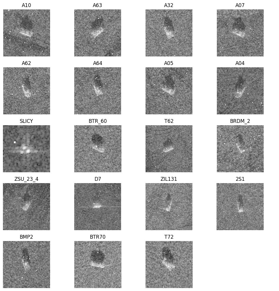
Displayed below are some examples for every class in the dataset. To plot them, we extracted only the magnitude of the signals although the data are indeed complex valued.
SAMPLE
SAMPLE is a dataset built from real SAR data as provided by the MSTAR dataset as well a synthetic data. As the original MSTAR dataset, it contains military vehicles and actually a subset of 10 classes : 2s1, bmp2, btr70, m1, m2, m35, m548, m60, t72, zsu23 . It contains a total of 3968 samples. The SAMPLE dataset is provided by https://github.com/benjaminlewis-afrl/SAMPLE_dataset_public .
- class torchcvnn.datasets.SAMPLE(rootdir: str, transform=None, download: bool = False)[source]
The SAMPLE dataset is made partly from real data provided by MSTAR and partly from synthetic data.
The dataset is public and will be downloaded if requested and missing on drive.
It is made of 10 classes of military vehicles: 2s1, bmp2, btr70, m1, m2, m35, m548, m60, t72, zsu23
- Parameters:
rootdir (str) – Path to the root directory where the dataset is stored or will be downloaded
transform (torchvision.transforms.Compose) – A list of torchvision transforms to apply to the complex image
download (bool) – Whether to download the data if missing on disk
Note
An example usage :
import torchcvnn
from torchcvnn.datasets import SAMPLE

transform = v2.Compose(
    transforms=[v2.ToImage(), v2.Resize(128), v2.CenterCrop(128)]
)
dataset = SAMPLE(
    rootdir, transform=transform, download=True
)
X, y = dataset[0]
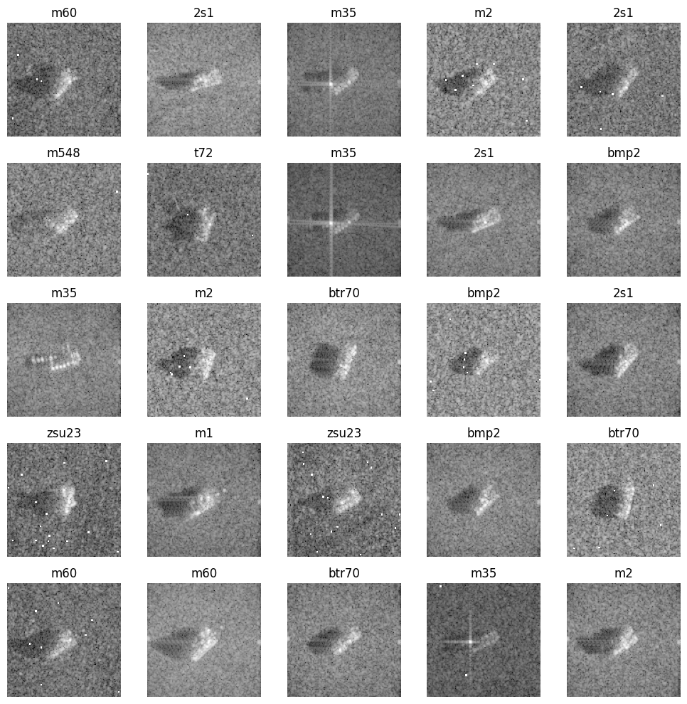
Displayed below are some examples drawn randomly from SAMPLE. To plot them, we extracted only the magnitude of the signals although the data are indeed complex valued.
MICCAI2023
The MICCAI2023 challenge involved the task of cine reconstruction where the objective is to predict a full sampled k-space from an under-sampled k-space. The data come from cardiac MRI.
- torchcvnn.datasets.miccai2023.kspace_to_image(kspace: Tensor | ndarray) Tensor[source]
Convert k-space data to image data. The returned kspace is of the same type than the the provided image (np.ndarray or torch.Tensor).
- Parameters:
kspace – torch.Tensor or np.ndarray k-space data
- Returns:
- torch.Tensor or np.ndarray
image data
- torchcvnn.datasets.miccai2023.image_to_kspace(img: Tensor | ndarray) Tensor | ndarray[source]
Convert image data to k-space data. The returned kspace is of the same type than the the provided image (np.ndarray or torch.Tensor)
- Parameters:
img – torch.Tensor or np.ndarray Image data
- Returns:
- torch.Tensor or np.ndarray
k-space data
- torchcvnn.datasets.miccai2023.combine_coils_from_kspace(kspace: ndarray) ndarray[source]
Combine the coils of the k-space data using the root sum of squares
- Parameters:
kspace – np.ndarray k-space data of shape (sc, ky, kx)
- Returns:
- np.ndarray
Image data with coils combined, of shape (ky, kx), real valued, positive
- class torchcvnn.datasets.MICCAI2023(rootdir: str, view: CINEView = CINEView.SAX, acc_factor: AccFactor = AccFactor.ACC4)[source]
Loads the MICCAI2023 challenge data for the reconstruction task Task 1
The data are described on https://cmrxrecon.github.io/Task1-Cine-reconstruction.html
You need to download the data before hand in order to use this class.
For loading the data, you may want to alternatively consider the fastmri library, see https://github.com/facebookresearch/fastMRI/
The structure of the dataset is as follows:
- rootdir/ChallengeData/MultiCoil/cine/TrainingSet/P{id}/
cine_sax.mat
cin_lax.mat
- rootdir/ChallengeData/MultiCoil/cine/TrainingSet/AccFactor04/P{id}/
cine_sax.mat
cine_sax_mask.mat
cin_lax.mat
cine_lax_mask.mat
- rootdir/ChallengeData/MultiCoil/cine/TrainingSet/AccFactor08/P{id}/
cine_sax.mat
cine_sax_mask.mat
cin_lax.mat
cine_lax_mask.mat
- rootdir/ChallengeData/MultiCoil/cine/TrainingSet/AccFactor10/P{id}/
cine_sax.mat
cine_sax_mask.mat
cin_lax.mat
cine_lax_mask.mat
The cine_sax or sine_lax files are \((k_x, k_y, s_c, s_z, t)\) where :
\(k_x\): matrix size in x-axis (k-space)
\(k_y`\): matrix size in y-axis (k-space)
\(s_c\): coil array number (compressed to 10)
\(s_x\): matrix size in x-axis (image)
\(s_y\): matrix size in y-axis (image) , used in single-coil data
\(s_z\): slice number for short axis view, or slice group for long axis (i.e., 3ch, 2ch and 4ch views)
\(t\): time frame.
Note the k-space dimensions (in x/y axis) are not the same depending on the patient.
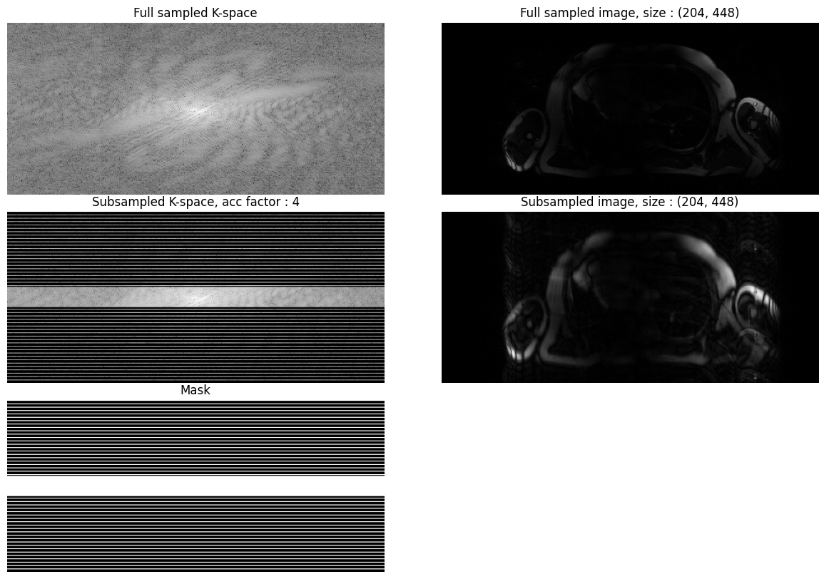
This is a recontruction dataset. The goal is to reconstruct the fully sampled k-space from the subsampled k-space. The acceleratation factor specifies the subsampling rate.
There are also the Single-Coil data which is not yet considered by this implementation
Note
An example usage :
import torchcvnn
from torchcvnn.datasets.miccai2023 import MICCAI2023, CINEView, AccFactor

def process_kspace(kspace, coil_idx, slice_idx, frame_idx):
    coil_kspace = kspace[:, :, coil_idx, slice_idx, frame_idx]
    mod_kspace = np.log(np.abs(coil_kspace) + 1e-9)

    img = kspace_to_image(coil_kspace)
    img = np.abs(img)
    img = img / img.max()

    return mod_kspace, img

dataset = MICCAI2023(rootdir, view=CINEView.SAX, acc_factor=AccFactor.ACC8)
subsampled_kspace, subsampled_mask, full_kspace = dataset[0]

frame_idx = 5
slice_idx = 0
coil_idx = 9

mod_full, img_full = process_kspace(full_kspace, coil_idx, slice_idx, frame_idx)
mod_sub, img_sub = process_kspace(subsampled_kspace, coil_idx, slice_idx, frame_idx)

# Plot the above magnitudes
...
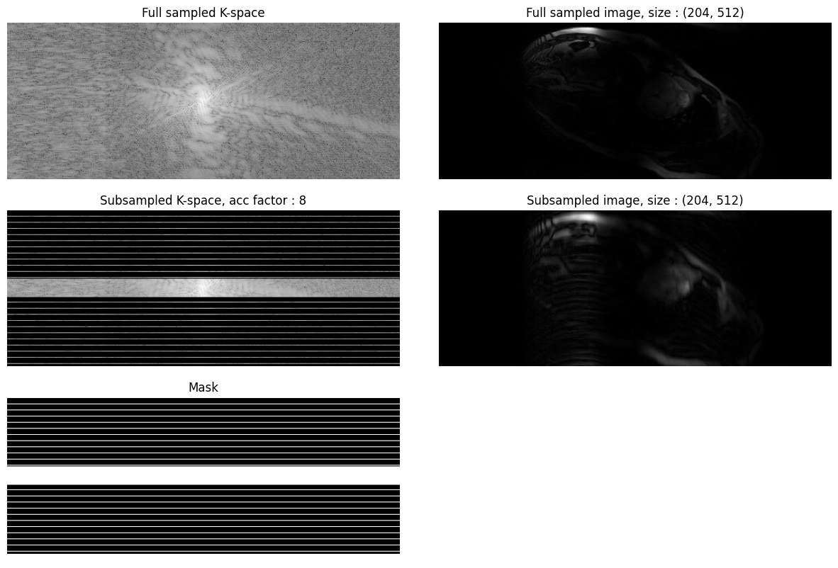
Displayed below is an example patient with the SAX view and acceleration of 8:
Displayed below is an example patient with the LAX view and acceleration of 4:
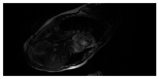
You can combine the coils using the root sum of squares to get a magnitude image (real valued) with all the coil contributions.
Below are examples combining the coils for a given frame and slice, for LAX (top) and SAX (bottom). It uses the function
torchcvnn.datasets.miccai2023.combine_coils_from_kspace()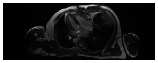
ATRNet-STAR
ATRNet-STAR is a large vehicule classification/detection dataset of SAR images provided by Liu et al.(2025) and released on huggingface hub (`https://huggingface.co/datasets/waterdisappear/ATRNet-STAR`_). It contains :
40 target types with 17003 training samples and 7243 test samples.
quad polarization
bands X, Ku
- class torchcvnn.datasets.ATRNetSTAR(root_dir: str, split: Literal['train', 'test', 'all'] | str, benchmark: str | None = None, download: bool = False, class_level: Literal['type', 'class', 'category'] = 'type', get_annotations: bool = False, transform: Callable | None = None)[source]
Implements a PyTorch Dataset for the ATRNet-STAR dataset presented in :
Yongxiang Liu, Weijie Li, Li Liu, Jie Zhou, Bowen Peng, Yafei Song, Xuying Xiong, Wei Yang, Tianpeng Liu, Zhen Liu, & Xiang Li. (2025). ATRNet-STAR: A Large Dataset and Benchmark Towards Remote Sensing Object Recognition in the Wild.
Only slant-range quad polarization complex images are supported.
The dataset is composed of pre-defined benchmarks (see paper). Dowloading them automatically is possible, but a Hugging Face authentification token is needed as being logged in is required for this dataset.
Warning : samples are ordered by type, shuffling them is recommended.
- Parameters:
root_dir (str) – The root directory in which the different benchmarks are placed. Will be created if it does not exist.
benchmark (str) – (optional) Chosen benchmark. If not specified, SOC_40 (entire dataset) will be used as default.
split (str) – Chosen split (‘train’, ‘test’, … or ‘all’ for all benchmark samples). Those are pre-defined by the dataset for each benchmark.
download (bool) – (optional) Whether or not to download the dataset if it is not found. Default: False
class_level (str) – (optional) The level of precision chosen for the class attributed to a sample. Either ‘category’, ‘class’ or ‘type’. Default: ‘type’ (the finest granularity)
get_annotations (bool) – (optional) If False, a dataset item will be a tuple (sample, target class) (default). If True, the entire sample annotation dictionnary will also be returned: (sample, target class, annotation dict).
transform (Callable) – (optional) A transform to apply to the data
